Options

Query and background samples

Composition Profiler provides an easy way to visually investigate bias in amino acid composition between two sets of protein sequences. A set of proteins under study (the query sample) can be analyzed against a representative sample of proteins from the organism under study, or a group of proteins with a contrasting functional annotation (the background sample), which provides a suitable background amino acid distribution.

Sequences should be entered in FastA format.

There are no theoretical limits on the number of sequences that can be given as input. Composition Profiler treats differences in amino acids composition as "signals" – since the p-value is a function of the sample size and signal strength, samples which are not large enough for the inherent signal will give differences with p-value above the statistical significance threshold, and will be discarded as spurious. With small sample sizes, only the strongest signals will be identified.

For example, if a sample consisting of only one sequence, AAAAAAAAAA, were to be analyzed against SwissProt, because the difference between 100% A in the sample and 7.89% A in SwissProt presents a very strong signal (12 fold enrichment), the difference will be statistically significant. Larger sample size allows identification of more subtle signals.

Background distribution

Alternatively, the query sample can be analyzed against one of the standard protein datasets:

• SwissProt 51 (Bairoch et al., 2005), closest to the distribution of amino acids in nature among the four datasets
• PDB Select 25 (Berman et al, 2000), a subset of structures from the Protein Data Bank with less than 25% sequence identity, biased towards the composition of proteins amenable to crystallization studies
• Surface residues determined by the Molecular Surface Package over a sample of PDB structures of monomeric proteins, suitable for analyzing phenomena on protein surfaces, such as binding
• DisProt 3.4, comprised of a set of consensus sequences of experimentally determined disordered regions (Sickmeier et al., 2007)

To illustrate the importance of choosing an appropriate background distribution, we generated composition profiles of (A) PDBS25, (B) surface residues dataset and (C) DisProt against SwissProt:

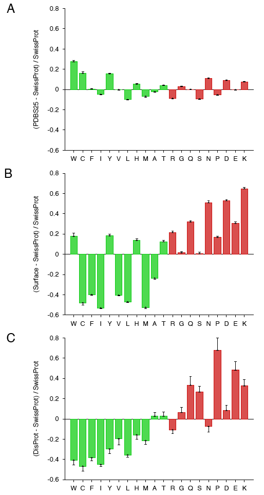
All three graphs have the same y-axis scale, the same order of amino acids and the same color-coding scheme (Vihinen flexibility), which allows direct visual comparison of the amino acid biases in the three datasets.

Discovery

Alpha value

Statistical significance of an observed enrichment or depletion is estimated using permutations. Concatenation of query and backround sequences is randomly permuted and a test statistic more extreme than the one observed in the actual data is counted towards the pvalue.

Any particular enrichment or depletion is statistically significant when the P-value is lower than or equal to a user-specified statistical significance (alpha) value.

Bonferroni correction

Simple multiple testing correction. Assumes independence of tests, and divides the alpha value by the total number of tests. See (Weisstein) for details.

Number of iterations

In the context of calculating composition differences, bootstrapping is used for non-parametric estimation of the confidence intervals for reported amino acid compositions. More precisely, reported confidence intervals are standard deviations of pseudo-replicate compositions.

In the context of discovery and relative entropy calculations, permutations are used to estimate the statistical significance of the observed test statistic (fractional difference or relative entropy). In each iteration, a random permutation of the two starting samples is created, the test statistic is computed based on the permuted sample and permutation test statistic more extreme than the observed test statistic is coutned towards the P-value.

Amino acid grouping, ordering and color-coding

Alpha helix frequency (Nagano, 1973)

Y	P	G	N	S	R	T	C	I	V	D	W	Q	L	K	M	F	A	H	E
0.63	0.70	0.72	0.77	0.78	0.83	0.87	0.94	0.94	0.97	1.00	1.06	1.10	1.23	1.23	1.23	1.23	1.29	1.29	1.54

Aromatics

Aromatic amino acids (F, W, Y) are colored green, and the remaining amino acids are colored black.

Beta structure frequency (Nagano, 1973)

E	R	N	P	S	K	H	D	G	A	Y	C	W	Q	T	L	M	F	V	I
0.33	0.67	0.72	0.75	0.77	0.81	0.87	0.9	0.9	0.96	1.07	1.13	1.13	1.18	1.23	1.26	1.29	1.37	1.41	1.54

Bulkiness (Zimmerman et al., 1968)

G	S	A	D	N	C	E	H	R	Q	K	T	M	P	Y	F	I	L	V	W
3.4	9.47	11.5	11.68	12.82	13.46	13.57	13.69	14.28	14.45	15.71	15.77	16.25	17.43	18.03	19.8	21.4	21.4	21.57	21.67

Charge

Positively charged residues (K, R) are colored blue, negatively charged residues (D, E) are colored red; and neutral residues are colored black.

Coil propensity (Nagano, 1973)

F	M	L	A	E	H	I	Q	V	K	W	C	T	D	R	S	G	Y	N	P
0.58	0.62	0.63	0.72	0.75	0.76	0.8	0.81	0.83	0.84	0.87	1.01	1.03	1.04	1.33	1.34	1.35	1.35	1.38	1.43

Disorder propensity (Dunker et al., 2001)

Disorder-promoting residues (A, R, S, Q, E, G, K, P ) are colored red, order-promoting residues (N, C, I, L, F, W, Y, V) are colored blue, and disorder-order neutral residues (D, H, M, T) are colored black.

Flexibility (Vihinen et al., 1994)

W	C	F	I	Y	V	L	H	M	A	T	R	G	Q	S	N	P	D	E	K
0.904	0.906	0.915	0.927	0.929	0.931	0.935	0.950	0.952	0.984	0.997	1.008	1.031	1.037	1.046	1.048	1.049	1.068	1.094	1.102

Hydrophobicity (Eisenberg et al., 1984)

R	K	D	Q	N	E	H	S	T	P	Y	C	G	A	M	W	L	V	F	I
-2.53	-1.5	-0.9	-0.85	-0.78	-0.74	-0.4	-0.18	-0.05	0.12	0.26	0.29	0.48	0.62	0.64	0.81	1.06	1.08	1.19	1.38

Hydrophobicity (Kyte and Doolittle, 1982)

R	K	D	E	N	Q	H	P	Y	W	S	T	G	A	M	C	F	L	V	I
-4.5	-3.9	-3.5	-3.5	-3.5	-3.5	-3.2	-1.6	-1.3	-0.9	-0.8	-0.7	-0.4	1.8	1.9	2.5	2.8	3.8	4.2	4.5

Hydrophobicity (Fauchere and Pliska, 1983)

R	K	D	E	N	Q	S	G	H	T	A	P	Y	V	C	L	F	I	M	W
-1.01	-0.99	-0.77	-0.64	-0.6	-0.22	-0.04	0.0	0.13	0.26	0.31	0.72	0.96	1.22	1.54	1.7	1.79	1.8	1.23	2.25

Interface propensity (Jones and Thornton, 1997)

D	K	S	P	T	A	E	Q	G	N	R	V	L	H	C	I	M	Y	F	W
-0.38	-0.36	-0.33	-0.25	-0.18	-0.17	-0.13	-0.11	-0.07	0.12	0.27	0.27	0.4	0.41	0.43	0.44	0.66	0.66	0.82	0.83

Linker propensity (George and Heringa, 2003)

C	G	W	D	I	N	K	S	V	A	Y	H	T	M	Q	E	L	F	R	P
0.778	0.835	0.895	0.916	0.922	0.944	0.944	0.947	0.955	0.964	1.0	1.014	1.017	1.032	1.047	1.051	1.085	1.119	1.143	1.299

Polarity (Zimmerman et al., 1968)

A	G	I	L	V	F	M	C	P	Y	T	S	W	N	Q	K	D	E	H	R
0.0	0.0	0.13	0.13	0.13	0.35	1.43	1.48	1.58	1.61	1.66	1.67	2.1	3.38	3.53	49.5	49.7	49.9	51.6	52.0

Size (Dawson, 1972)

G	A	D	C	S	N	E	T	V	I	L	P	Q	H	M	F	K	W	Y	R
0.5	2.5	2.5	3.0	3.0	5.0	5.0	5.0	5.0	5.5	5.5	5.5	6.0	6.0	6.0	6.5	7.0	7.0	7.0	7.5

Surface exposure (Janin, 1979)

K	R	E	Q	D	N	Y	P	T	H	S	A	G	W	M	L	F	V	I	C
-1.8	-1.4	-0.7	-0.7	-0.6	-0.5	-0.4	-0.3	-0.2	-0.1	-0.1	0.3	0.3	0.3	0.4	0.5	0.5	0.6	0.7	0.9

Solvation potential (Jones and Thornton, 1996)

W	F	I	L	M	Y	V	C	H	A	G	S	T	P	N	R	Q	D	E	K
-0.68	-0.55	-0.49	-0.49	-0.40	-0.32	-0.31	-0.30	-0.06	0.05	0.08	0.15	0.16	0.19	0.22	0.41	0.45	0.64	0.77	1.61

Additional color schemes

WebLogo default colors

Amino Acid	Color Name	RGB	Hexadecimal
G, S, T, Y, C	green	[0,204,0]	00CC00
N, Q	purple	[204,0,204]	CC00CC
K, R, H	blue	[0,204,0]	0000CC
D, E	red	[204,0,0]	CC0000
P,A,W,F,L,I,M,V	black	[0,0,0]	000000

Amino Colors

Amino Acid	Color Name	RGB	Hexadecimal
D, E	bright red	[230,10,10]	E60A0A
C, M	yellow	[230,230,0]	E6E600
K, R	blue	[20,90,255]	145AFF
S, T	orange	[250,150,0]	FA9600
F, Y	mid blue	[50,50,170]	3232AA
N, Q	cyan	[0,220,220]	00DCDC
G	light grey	[235,235,235]	EBEBEB
L, V, I	green	[15,130,15]	0F820F
A	dark grey	[200,200,200]	C8C8C8
W	pink	[180,90,180]	B45AB4
H	pale blue	[130,130,210]	8282D2
P	flesh	[220,150,130]	DC9682

Shapley color table

Amino Acids	Color Name	RGB	Hexadecimal
D, T	dark red	[160,0,66]	A00042
E	red-brown	[102,0,0]	660000
C	bright yellow	[255,255,112]	FFFF70
M, Y	dark yellow	[184,160,66]	B8A042
K	blue	[71,71,184]	4747B8
R	dark blue	[0,0,124]	00007C
S, Q	orange	[255,76,76]	FF4C4C
F, P, W	dark grey	[83,76,66]	534C42
N	flesh	[255,124,112]	FF7C70
G, V	light grey	[235,235,235]	EBEBEB
I	dark green	[0,76,0]	004C00
L	grey-green	[69,94,69]	455E45
A	light green	[140,255,140]	8CFF8C
H	pale blue	[112,112,255]	7070FF

In the original Shapley scheme, G and V are color-coded as white. Since this would render them invisible against a white background, their color has been changed to light grey.

Show Y-axis label

Shows label on the Y-axis of the profile graph.

Output format

Composition Profiler supports:

• Portable Network Graphics (PNG)
• Portable Document Format (PDF)
• Encapsulated PostScript (EPS)

Additionally, raw values for bar heights and error bars are displayed if plain text (TXT) option is chosen.

Output size

Height and width of the output image, in pixels, centimeters or inches.

Resolution

Sets up the image resolution. Applicable to bitmaps only (PNG).

References

• Bairoch A, Apweiler R, Wu CH, Barker WC, Boeckmann B, Ferro S, Gasteiger E, Huang H, Lopez R, Magrane M, Martin MJ, Natale DA, O'Donovan C, Redaschi N, and Yeh LS. (2005) "The Universal Protein Resource (UniProt)." Nucleic Acids Research 33:D154-159.
• Berman HM, Westbrook J, Feng Z, Gilliland G, Bhat TN, Weissig H, Shindyalov IN, and Bourne PE. (2000) "The Protein Data Bank." Nucleic Acids Research, 28:235-242.
• Dawson DM. (1972) In The Biochemical Genetics of Man (Brock DJH and Mayo O, eds.), Academic Press, New York, 1-38.
• Dunker AK, Lawson JD, Brown CJ, Williams RM, Romero P, Oh JS, Oldfield CJ, Campen AM, Ratliff CM, Hipps KW et al. (2001) "Intrinsically disordered protein." J. Mol. Graph. Model., 19, 26-59.
• Eisenberg D, Schwarz E, Komaromy M, and Wall R. (1984) "Analysis of membrane and surface protein sequences with the hydrophobic moment plot." J. Mol. Biol. 179:125-142.
• Fauchere J-L, and Pliska VE. (1983) "Hydrophobic parameters pi of amino acid side chains from partitioning of N-acetyl-amino-acid amides." Eur. J. Med. Chem. 18:369-375.
• George RA, and Heringa J. (2003) An analysis of protein domain linkers: their classification and role in protein folding. Protein Eng. 15:871-879.
• Hogg RV and Craig A. (1994) Introduction to Mathematical Statistics, 5th edition, Prentice Hall.
• Janin J. (1979) "Surface and inside volumes in globular proteins." Nature, 277, 491-492.
• Jones S, and Thornton J. (1997) "Analysis of protein-proteins interaction sites using surface patches." J. Mol. Biol. 272:121-132.
• Jones S, and Thornton J. (1996) "Principles of protein-protein interactions." Proc. Natl. Acad. Sci. USA, 93:13-20.
• Kyte J, and Doolittle RF. (1982) "A simple method for displaying the hydropathic character of a protein." J. Mol. Biol. 157:105-132.
• Nagano K. (1973) "Local analysis of the mechanism of protein folding. I. Prediction of helices, loops, and beta-structures from primary structure." J. Mol. Biol. 75:401-420.
• Sickmeier M, Hamilton JA, LeGall T, Vacic V, Cortese MS, Tantos A, Szabo B, Tompa P, Chen J, Uversky VN, Obradovic Z, and Dunker AK. (2007) "DisProt: the Database of Disordered Proteins." Nucleic Acids Research. 35:D786-93.
• Vihinen M, Torkkila E, and Riikonen P. (1994) "Accuracy of protein flexibility predictions." Proteins, 19, 141-149.
• Weisstein EW. "Bonferroni Correction." From MathWorld - A Wolfram Web Resource. http://mathworld.wolfram.com/BonferroniCorrection.html
• Zimmerman JM, Eliezer N, and Simha R. (1968) "The characterization of amino acid sequences in proteins by statistical methods." J J. Theor. Biol. 21:170-201.